Classification

Often we are given the task, from ourselves or from others, to label things according to a set of already existing classes:

• Is the object in the image a vehicle or a cat?
• Is this animal a dog or a cat?

Classification is the problem of giving the right label to a record given as input. The task is different from regression because here we have discrete labels instead of continuous values [SKIENA2017]. In this chapter we’ll give a brief introduction on binary and multi-class classification tasks and show how to tackle these problems using UFJF-MLTK.

Add #include <ufjfmltk/Classification.hpp> to include the classification module.

Binary classification

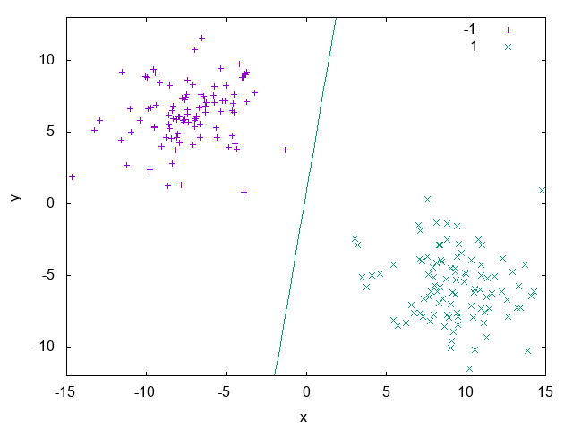
Fig. 14 Example of a binary classification problem with a linear discriminant.

Let \(Z = (x_{i}, y_{i})\) be a set of samples of size \(m\), where \(x_{i} \in R^{d}\), called input space of the problem, \(y_{i}\) is a scalar representing the class of each vector \(x_{i}\) and for binary classification \(y_{i} \in \{+1,-1\}\), for \(i = \{1, \dots, m\}\). A linear classifier, in a linearly separable input space, is represented by a hyperplane with the following equation [VILLELA2011]:

\[h(x) = \langle w, x \rangle + b\]

The classification result can be obtained through a signal function \(\varphi\) applied to the discriminant value associated to the hyperplane equation, i.e:

\[\begin{split}\varphi (h(x)) = \begin{cases} +1,& \text{if } h(x) \geq 0\\ -1,& \text{otherwise} \end{cases}\end{split}\]

The Perceptron algorithm

Considered the first learning algorithm, the Perceptron model is a pattern recognition model proposed by [ROSENBLATT1958]. It’s structured by a input layer connecting each input unit to a component from a \(d\)-dimension vector, and a output layer composed of \(m\) units. Therefore, it’s an artificial neural network model with only one processing layer. In its simplest form, the Perceptron algorithm is a classification algorithm involving only two classes [VILLELA2011].

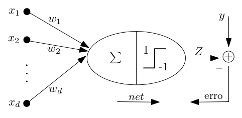
Fig. 15 Perceptron model topology.

The algorithm developed by Rosenblatt can be utilized to determine the \(w\) vector in a limited number of iterations, where the number of iterations is related to the number of updates of the weights vector. As the weights vector \(w\) is determined by successive corrections in order to minimize a loss function, we can say that the separating hyperplane is constructed in a iterative way characterizing an online learning process [VILLELA2011].

Listing 1 Primal Perceptron example

#include <ufjfmltk/ufjfmltk.hpp>

namespace vis = mltk::visualize;
namespace classifier = mltk::classifier;

int main() {
    mltk::Data<double> data("iris.data");
    vis::Visualization<> vis(data);
    classifier::PerceptronPrimal<double> perceptron(data);

    perceptron.train();

    vis.plot2DwithHyperplane(1, 2, perceptron.getSolution(), true);
}

On Listing 1 we can see a simple usage of the UFJF-MLTK perceptron implementation in it’s primal form. In this example we first load the binary iris.data dataset where two of the three original classes were merged into one in order to generate a binary problem, after that we instantiate the PerceptronPrimal wrapper with the same data type as the dataset and the default parameters. With the object from the algorithm wrapper we call the method train to learn a model from the data and, finally, the decision boundary is ploted with features 1 and 2 from the dataset and passing the perceptron solution. Fig. 16 shows the hyperplane generated by the model.

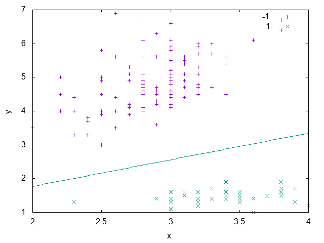
Fig. 16 Solution generated from the model trained by the Perceptron classifier.

Kernel methods

Often in real datasets is not possible to do a linear separation of the data. In these cases is necessary to utilize more complex functions for labels separation. One way to define a non-linear separator is through a mapping function from input space \(X\) to a higher dimensional space where the separation is possible [MEHRYAR2018].

In models based on a mapping from the fixed non-linear features space \(\Phi(x)\), the kernel function is defined as following [BISHOP2007]:

(1)\[k(x, x^{'}) = \Phi(x)^{T}\Phi(x^{'})\]

Fig. 17 shows an example of a dataset that isn’t linearly separable. It’s composed of two spirals and as we can see, there isn’t a way to draw a line that separates the samples belonging to each spiral. In the Dual Perceptron section we’ll see how to solve this problem.

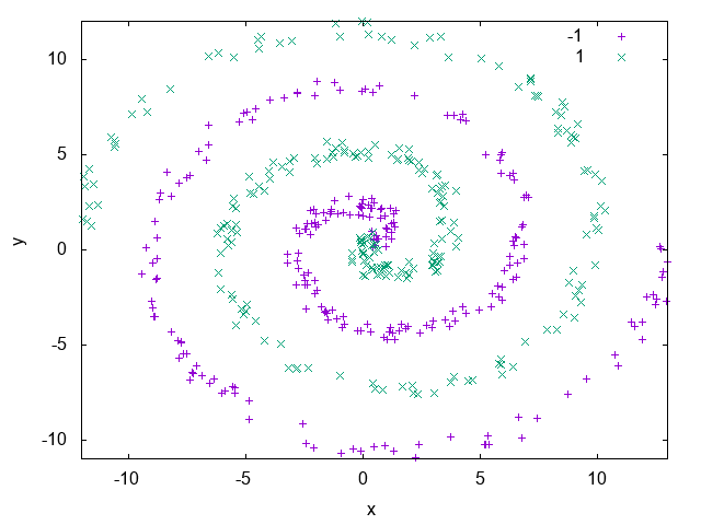
Fig. 17 Spirals artificial dataset.

The simplest kernel considering the mapping on Eq. (1) is the linear kernel where \(\Phi(x) = x\) and \(k(x, x^{'}) = x^{T}x\). The kernel concept formulated as a inner product in the input space allows the generalization of many known algorithms. The main idea is that if an algorithm is formulated in such a way that the input vector \(x\) is presented in a scalar product form, the inner product can be replaced by another kernel product. This kind of extension is known as kernel trick or kernel substitution [BISHOP2007].

The Perceptron dual algorithm

The derivation and implementation of the dual form of the Perceptron algorithm will be shown in Section ??, since it’s a more complex topic. For now, we’ll use UFJF-MLTK implementation to solve the spirals dataset problem presented earlier.

Listing 2 Dual perceptron training on spirals artificial dataset.

  #include <ufjfmltk/ufjfmltk.hpp>

  namespace vis = mltk::visualize;
  namespace classifier = mltk::classifier;

  int main() {
      auto data = mltk::datasets::make_spirals(500);
      vis::Visualization<> vis(data);
      classifier::PerceptronDual<double> perceptron(data, mltk::KernelType::GAUSSIAN, 1);

      perceptron.setMaxTime(500);
      perceptron.train();

      vis.plotDecisionSurface2D(perceptron, 0, 1, true, 100);
  }

Listing 2 example generates a spirals dataset with 500 samples using the make_spirals function from mltk::datasets:: namespace, initialize the visualization object and instantiate the PerceptronDual wrapper with a gaussian kernel with standard deviation of 1.0 as a kernel parameter. To guarantee the algorithm convergence, the maximum training time of the algorithm is set as 500ms, after that, the model is trained and its decision boundary is ploted as in Fig. 18.

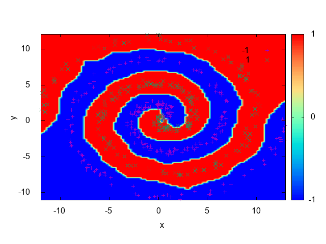
Fig. 18 Decision contour surface from Perceptron dual for spirals dataset.

Multi-class classification

Until now we’ve been discussing algorithms for classification problems were we have only two labels, but often we face problems where we need to choose a class between tens, hundreds or even thousands of labels, like when we need to assign a label to an object in an image. In this chapter, we’ll be analysing the problem of multi-class classification learning.

Let \(\mathcal{X}\) be the input space and \(\mathcal{Y}\) the output space, and let \(\mathcal{D}\) be an unknown distribution over \(\mathcal{X}\) according to which input points are drawn. We’ll be distinguishing between the mono-label (binary classification) and multi-label cases, where we define \(\mathcal{Y}\) as a set of discrete values as \(\mathcal{Y} = \{1, \dots, k\}\) and \(\mathcal{Y} = \{+1, -1\}^{k}\) for the mono-label and multi-label cases, respectively. In the mono-label case, each sample will be assigned to only one class, while in the multi-label there can be several. The latter can be illustrated as the positive value being the component of a vector representing the classes where the example is associated [MEHRYAR2018].

On both cases, the learner receives labeled samples \(\mathcal{S} = ((x_1, y_1), \dots, (x_m, y_m)) \in (\mathcal{X}, \mathcal{Y})^{m}\) with \(x_1, \dots, x_m\) drawn according to \(\mathcal{D}\), and \(y_i = f(x_i)\) for all \(i \in [1, \dots, m]\), where \(f:\mathcal{X} \rightarrow \mathcal{Y}\) is the target labeling function. The multi-class classification problem consists of using labeled data \(\mathcal{S}\) to find a hypothesis \(h \in H\), where \(H\) is a hypothesis set containing functions mapping \(\mathcal{X}\) to \(\mathcal{Y}\). The multi-class classification problem consists on finding the hypothesis \(h \in H\) using the labeled data \(\mathcal{S}\), such that it has smallest generalization error \(R(h)\) with respect to the target \(f\), where Eq. (2) refers to the mono-label case and Eq. (3) to the multi-label case [MEHRYAR2018].

(2)\[R(h) = \mathop{\mathbb{E}}_{x \sim \mathcal{D}} [1_{h(x) \neq f(x)}]\]

(3)\[R(h) = \mathop{\mathbb{E}}_{x \sim \mathcal{D}} [\sum_{l=1}^{k} 1_{[h(x)]_l \neq [f(x)]_l}]\]

In the following sections we’ll be discussing two algorithms for adapting models for binary classification to the multi-class case, namely One-vs-All and One-vs-One. For that, the blobs artificial dataset generated with 50 examples for each of 3 labels. The plot for the dataset data can be seen on Fig. 19.

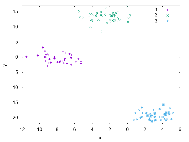
Fig. 19 Blobs artificial dataset.

The One-vs-All algorithm

This method consists in learning \(k\) binary classifiers \(h_l:\mathcal{X} \rightarrow {-1, +1}\), \(l \in \mathcal{Y}\), each one of them designed to discriminate one class from all the others. Each \(h_l\), for any \(l \in \mathcal{Y}\), is constructed by training a binary classifier after relabeling points in class \(l\) with 1 and all the others as -1 on the full sample \(\mathcal{S}\). The multi-class hypothesis \(h:\mathcal{X} \rightarrow \mathcal{Y}\) defined by the One-vs-All (OVA) technique is given by [MEHRYAR2018]:

\[\forall x \in \mathcal{X},\; h(x) = \mathop{arg\,max}_{l\in\mathcal{Y}}f_l(x)\]

Listing 3 shows how to use the UFJF-MLTK primal perceptron implementation with the OVA technique to tackle the blobs dataset classification problem. As can be seen, the only thing needed to do is to instantiate the OneVsAll wrapper and pass the training data and the algorithm wrapper to be used. Something to be noted, is that the base algorithm parameters must be passed on its initialization or before calling the OVA train method.

Listing 3 OVA example with the primal perceptron model.

  #include <ufjfmltk/ufjfmltk.hpp>

  namespace vis = mltk::visualize;
  namespace classifier = mltk::classifier;

  int main() {
      auto data = mltk::datasets::make_blobs(50, 3, 2, 1.5, -20, 20, true, true, 10).dataset;
      vis::Visualization<> vis(data);
      classifier::PerceptronPrimal<double> perceptron;
      classifier::OneVsAll<double> ova(data, perceptron);

      ova.train();

      vis.plotDecisionSurface2D(ova, 0, 1, true, 100, true);
  }

Fig. 20 shows the decision boundary generated after training, it’s possible to note that each region drawn accomodates points with the same class, indicating that the technique was effective on learning a aproximation of the data distribution. For non linearly separated data, the only changes is that we need to use an algorithm capable of learning a non-linear function like the dual perceptron from PerceptronDual wrapper.

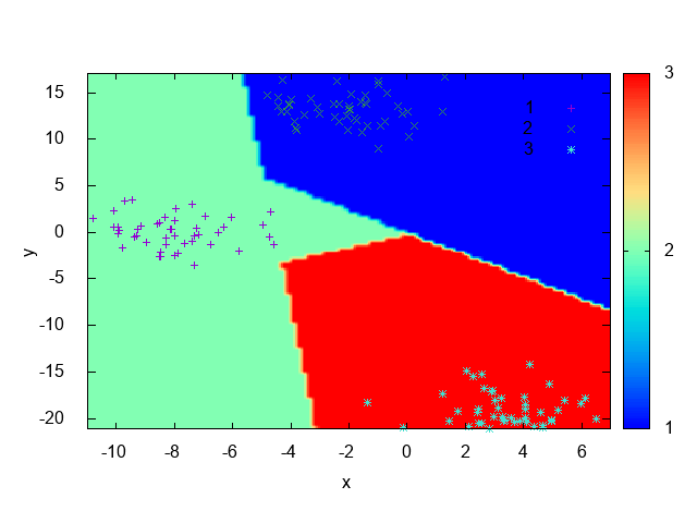
Fig. 20 Decision contour surface from OVA with perceptron for blobs dataset.

The One-vs-One algorithm

The One-vs-One (OVO) technique consists in learning a binary classifier \(h_{ll^{'}}:\mathcal{X}\rightarrow {-1, +1}\) for each pair of distinct classes \((l, l^{'}) \in \mathcal{Y}\), \(l \neq l^{'}\), discriminating \(l\) and \(l^{'}\). \(h_{ll^{'}}\) is obtained by training a binary classifier on the sub-sample containing exactly the points labeled as \(l\) and \(l^{'}\), with the value +1 returned for \(l^{'}\) and -1 for \(l\). For that, it’s needed to train \(\binom{k}{2} = \frac{k(k-1)}{2}\) classifiers, which are combined to define a multi-class classification hypothesis \(h\) via majority vote [MEHRYAR2018]:

\[\forall x \in \mathcal{X},\; h(x) = \mathop{arg\,max}_{l^{'} \in \mathcal{Y}}| \{l:h_{ll^{'}}(x) = 1\} |\]

Listing 4 OVO example with the primal perceptron model.

  #include <ufjfmltk/ufjfmltk.hpp>

  namespace vis = mltk::visualize;
  namespace classifier = mltk::classifier;

  int main() {
      auto data = mltk::datasets::make_blobs(50, 3, 2, 1.5, -20, 20, true, true, 10).dataset;
      vis::Visualization<> vis(data);
      classifier::PerceptronPrimal<double> perceptron;
      classifier::OneVsOne<double> ovo(data, perceptron);

      ovo.train();

      vis.plotDecisionSurface2D(ovo, 0, 1, true, 100, true);
  }

Listing 4 is analogous to Listing 3 except that it’s using the OneVsOne wrapper instead of the OVA one. As expected, it could also learn the data distribution, this can be seen by the decision boundary shown at Fig. 21.

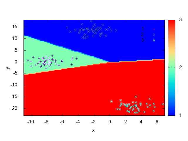
Fig. 21 Decision contour surface from OVO with perceptron for blobs dataset.

Model evaluation and selection

So far, you may have been able to build a classifier, but only that is not enough. Supose you’ve trained a model to predict the purchasing behavior of future clients using data from previous sales. For that, you need to estimate how accurately your model can be on unseen data, i.e, how accurately your model can predict the behavior of future customers. You may have built several classifiers and need to compare how well they can be between each other [HAN2011]. This section address metrics that can be used to compare those methods and how reliable this comparison can be.

Metrics for classifiers evaluation

The usage of training data for accuracy estimation of a classifier, can lead to overoptimistic estimates due to overspecialization of the model to the data. A better option to avoid this issue is to measure the classifier accuracy using a test set, that is are examples from the entire dataset that weren’t used during model training [HAN2011].

In this section we’ll be discussing several metrics to measure a classifier performance, but before we need to be confortable with some terminologies that’ll be used throghout metrics definitions. Two important terms are positive samples, points labeled with the class of main interest, and negative samples, that are the rest of the samples. Given two classes, for example, the positive samples may be buy_computer = yes and the negative samples buy_computer = no. Supose a classifier is used on a test set of labeled data. \(P\) is the number of positive samples and \(N\) is the number of negative samples. for each sample we compare For each sample, we compare the predictions made by the classifier with the sample known class. There are four other terms that must be understood since they are the building blocks of many evaluation measures computations [HAN2011].

• True positives (TP): positive samples that were correctly labeled by the classifier;
• True negatives (TN): negative samples that were correctly labeled by the classifier;
• False positives (FP): positive samples that were incorrectly labeled as negative;
• False negatives (FN): negative samples that were incorrectly labeled as positive.

A confusion matrix is a tool used to analyse if the classifier is doing well on prediction of examples of different classes. TP and TN indicates if the classifier is labeling right. FN and FP tells when the classifier is doing wrong predictions. These terms are sumarized on the confusion matrix from Table 1. It’s a matrix at least of size m x m where m is the number of classes, an entry \(CM_{ij}\) represents the number of examples from class \(i\) that were labeled as \(j\) [HAN2011].

Table 1 Confusion matrix where the lines represent the actual class and the columns the predicted class.

	yes	no
yes	TP	FN
no	FP	TN
Total	P’	N’

Below is a list of important metrics for classifiers evaluation and selection:

• Accuracy: percentage of examples on the test set that were correctly classified.

\[accuracy = \frac{TP + TN}{P + N}\]

• Error rate: is \(1 - accuracy(M)\) where \(accuracy(M)\) is the accuracy of the classifier \(M\). It can also be computed as follows:

\[error\;rate = \frac{FP + FN}{P + N}\]

• Sensitivity and Specificity: are the proportion of the positive samples that were correctly classified and the true negative proportion, respectively.

\[ \begin{align}\begin{aligned}sensitivity = \frac{TP}{P}\\specificity = \frac{TN}{N}\end{aligned}\end{align} \]

• Precision: can be thought as a measure of exactness, i.e, the percentage of examples labeled as positive are actually such.

\[precision = \frac{TP}{TP + FP}\]

• Recall: is a measure of completeness, i.e, the percentage of positive samples labeled as such, the same as sensitivity.

\[recall = \frac{TP}{TP + FN}\]

• F-score: can be viewed as a weighted average of the precision and recall. It reaches its best value at 1 and the worst at zero. Both precision and recall have the same contribution to the F-score.

\[F-score = \frac{2(precision * recall)}{precision + recall}\]

Listing 5 metrics computation for KNN classifier on spirals dataset.

#include <iostream>
#include <ufjfmltk/ufjfmltk.hpp>

namespace classifier = mltk::classifier;
namespace valid = mltk::validation;

int main() {
    auto data = mltk::datasets::make_spirals(500, 3, true, 2);
    valid::TrainTestPair traintest = valid::partTrainTest(data, 3);
    classifier::KNNClassifier<double> knn(traintest.train, 3);

    auto cfm = valid::generateConfusionMatrix(traintest.test, knn);
    valid::ValidationReport report = valid::metricsReport(traintest.test, cfm);

    std::cout << "True positive = " << report.tp << std::endl;
    std::cout << "True negative = " << report.tn << std::endl;
    std::cout << "False positive = " << report.fp << std::endl;
    std::cout << "False negative = " << report.fn << std::endl;
    std::cout << "Errors = " << report.errors << std::endl;
    std::cout << "Accuracy = " << report.accuracy*100.0 << std::endl;
    std::cout << "Error = " << report.error*100.0 << std::endl;

    mltk::utils::printConfusionMatrix(data.classes(), data.classesNames(), cfm);
}

Listing 5 shows how to compute some of the earlier mentionated metrics. On Lines 8-10 the program generates an instance of the spirals artificial dataset, split the data in training and test sets (see the next section) and create an object of the KNN classifier algorithm wrapper. After that, on Lines 12-13 the confusion matrix cfm is generated to be used by the metricsReport method, that evaluate the metrics of the model on the passed data and returns it as a ValidationReport object. From Line 15 to 21 some metrics are printed and, finally, the program prints the confusion matrix on the screen and exits.

Holdout method and random subsampling

With the holdout method the data is randomly partitioned in two independent sets, the training set and the test set. Usually, two thirds of the data is reserved for training and one third for testing. The training set is used to train the model and the test set for estimating the accuracy. The problem of this method is that it usually pessimistic because only a portion of the data is used to derive the model. The holdout accuracy estimation process is illustrated in Fig. 22 [HAN2011].

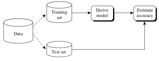
Fig. 22 Accuracy estimation with the holdout method.

Random subsampling is a variation of the holdout method where the holdout method is repeated \(k\) times. The accuracy estimate is given as the average of the accuracies obtained from each iteration [HAN2011].

Listing 6 loads the iris dataset for a multi-class classification task and splits the dataset in a training and test set pair. The data split is done dividing the data, in a stratified manner by default, in 3 folds and selects one of them for the test set and merge the other ones into a training set. After the data split, the OVA wrapper is instantiated with an object from the perceptron wrapper and the training set. Finally, the model is trained and the accuracy is estimated on the test set.

Listing 6 holdout accuracy estimation on iris dataset.

#include <iostream>
#include <ufjfmltk/ufjfmltk.hpp>

namespace classifier = mltk::classifier;
namespace valid = mltk::validation;

int main() {
    mltk::Data<> data("iris_mult.csv");
    valid::TrainTestPair traintest = valid::partTrainTest(data, 3);
    classifier::PerceptronPrimal<double> perc;
    classifier::OneVsAll<double> ova(traintest.train, perc);

    ova.train();

    std::cout << "Accuracy = " << valid::accuracy(traintest.test, ova) * 100.0 << std::endl;
}

Cross-validation

In k-fold cross-validation the data is partitioned in \(k\) mutually independent sets or folds \(D_1, D_2, ..., D_k\) of approximately equal size, performing training and testing \(k\) times. On each iteration \(i\) the i-th partition is used as test set and the \(k-1\) remaining partitions as training data. Unlike the holdout and random subsampling methods, here the folds are used for training k times and once for testing. For classification, the accuracy is given by the number of correct classifications divided by the total number of samples on the initial data [HAN2011].

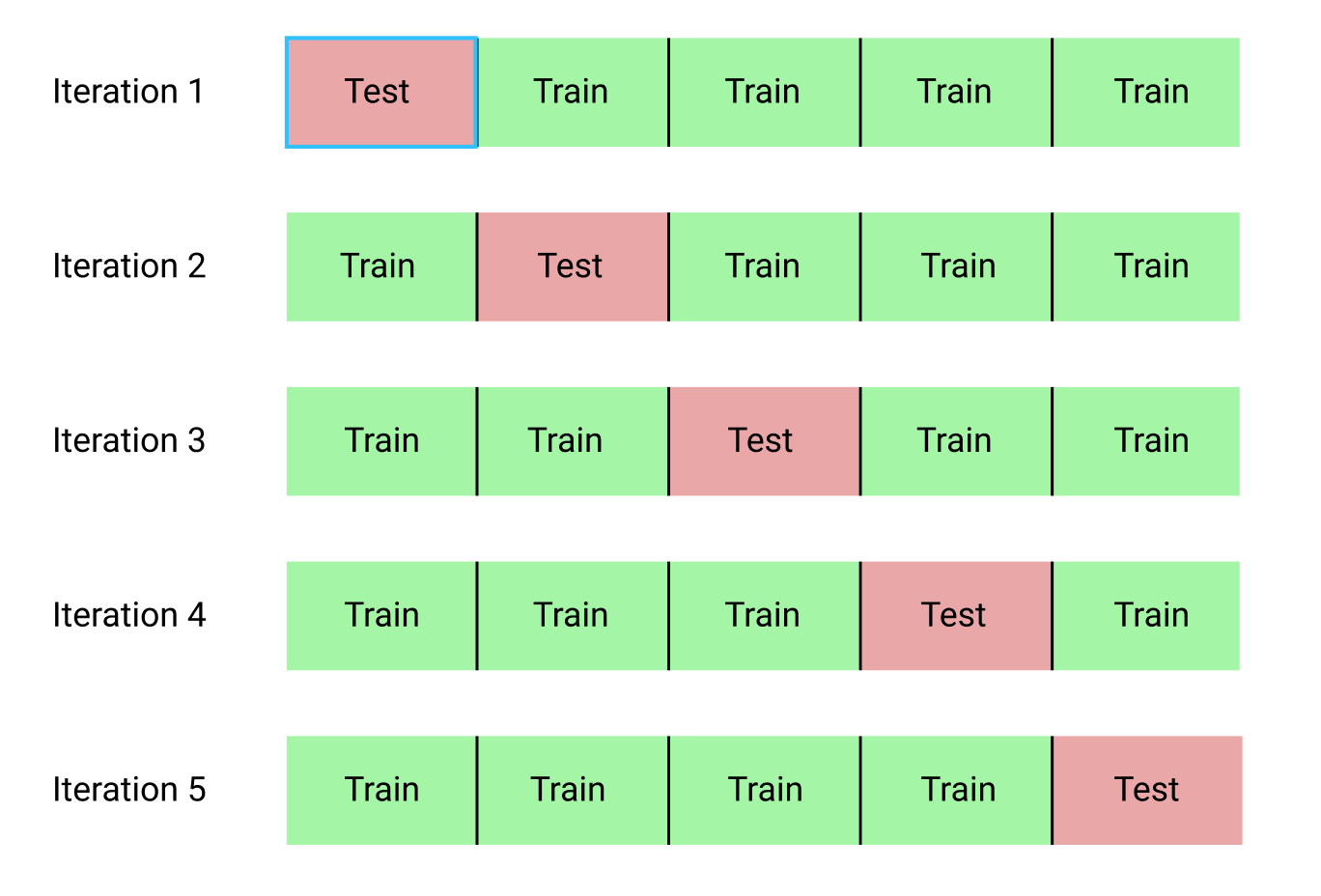
Fig. 23 k-fold cross validation process. Source: Towards data science

Leave-one-out is a special case from k-fold cross-validation where k is set as the total number of samples, i.e, only one sample is used as test set. In stratified cross-validation the folds are stratified so the distribution of the data is approximately equal to the initial data distribution. In general, 10-fold cross validation is recommended for accuracy estimation due its low bias and variance [HAN2011].

Listing 7 k-fold cross-validation accuracy estimation on iris dataset.

#include <iostream>
#include <ufjfmltk/ufjfmltk.hpp>

namespace classifier = mltk::classifier;
namespace valid = mltk::validation;

int main() {
    mltk::Data<> data("iris_mult.csv");
    classifier::PerceptronPrimal<double> perc;
    classifier::OneVsAll<double> ova(data, perc);

    valid::ValidationReport report = valid::kfold(data, ova, 10);

    std::cout << "Accuracy = " << report.accuracy << std::endl;
}

Listing 7 loads the iris dataset for a multi-class classification task and instantiate the OVA wrapper with a perceptron wrapper object. After that, it calls the k-fold cross-validation, stratified by default, with \(k=10\) on OVA with all the dataset data generating a report with metrics from k-fold. Finally, it prints the k-fold accuracy on the screen.

[SKIENA2017]

Skiena, Steven S. The data science design manual. Springer, 2017.

[VILLELA2011]

(1, 2, 3) Villela, Saulo Moraes, et al. “Seleção de Características utilizando Busca Ordenada e um Classificador de Larga Margem.” (2011).

[ROSENBLATT1958]

Rosenblatt, Frank. “The perceptron: a probabilistic model for information storage and organization in the brain.” Psychological review 65.6 (1958): 386.

[MEHRYAR2018]

(1, 2, 3, 4, 5) Mohri, Mehryar, Afshin Rostamizadeh, and Ameet Talwalkar. Foundations of machine learning. MIT press, 2018.

[BISHOP2007]

(1, 2) Bishop, Christopher M. “Pattern recognition and machine learning (information science and statistics).” (2007).

[HAN2011]

(1, 2, 3, 4, 5, 6, 7, 8) Han, Jiawei, Jian Pei, and Micheline Kamber. Data mining: concepts and techniques. Elsevier, 2011.